Recently, I wrote about the process capability index and tolerance interval. In today’s post, I am writing about the relationship between process capability index and sigma. The sigma number here relates to how many standard deviations the process window can hold.
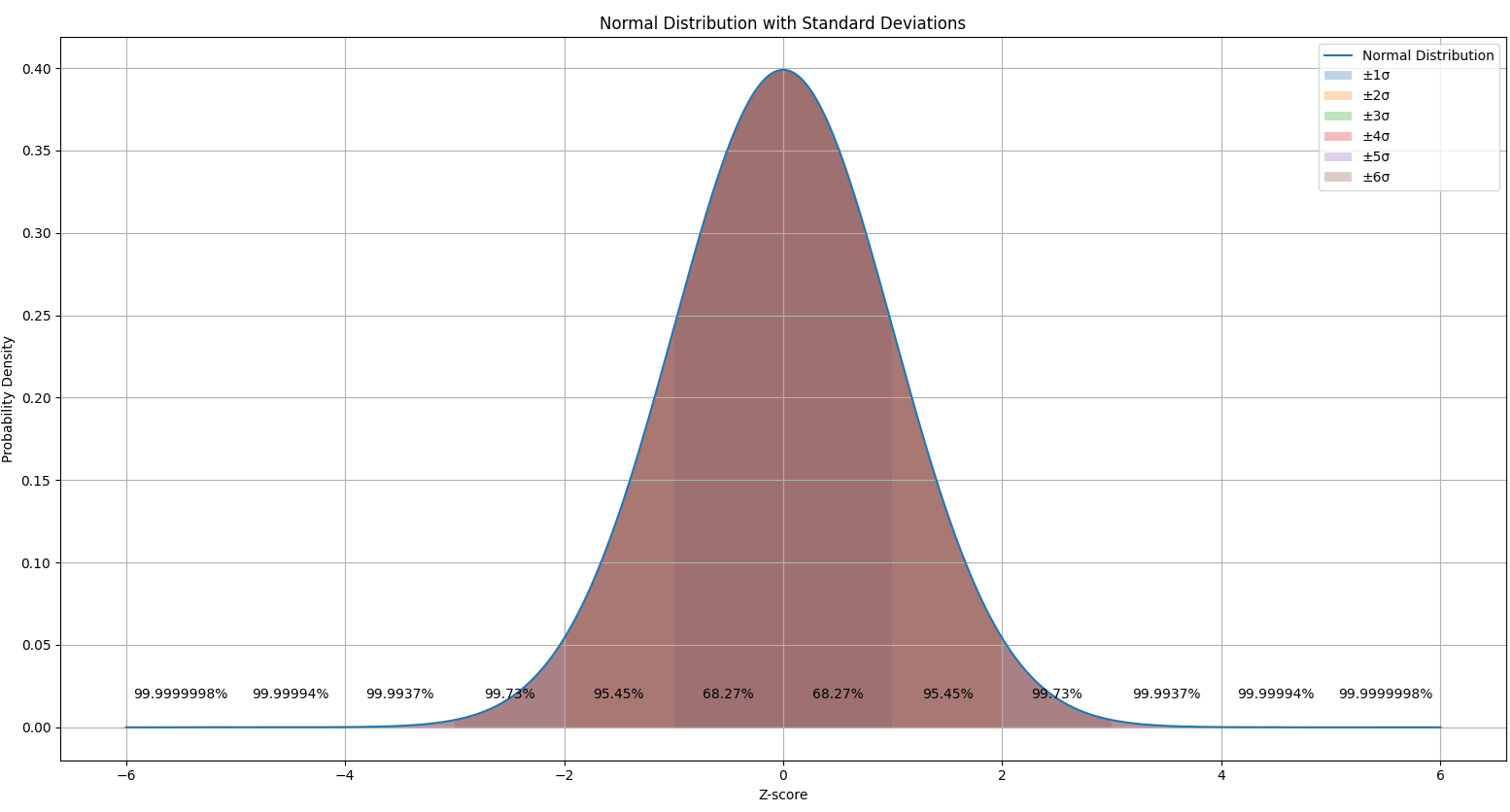
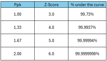
A +/- 3 sigma contains 99.73% of the normal probability density curve. This is also traditionally notated as the “process window”. The number of sigma’s is also the z-score. When the process window is compared against the specification window, we can assess the process capability. When the process window is much narrower than the specification window and is fully contained within the specification window, we say that the process is highly capable. When the process window is larger than the specification window, we say that the process is not capable. How much the process window is enclosed within the process specification window is explained by the process capability index. The most common process capability index is Cpk or Ppk. Here, we will consider Ppk.
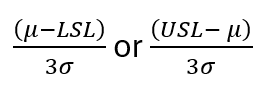
Ppk is the minimum of two values:
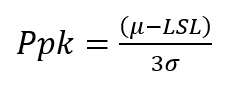
Here µ is the mean, σ is the standard deviation, LSL is the Lower Specification Limit, and USL is the Upper Specification Limit. We are splitting the process window into two here, and accounting for how centered the process is. If the process window is not centered compared to the process specification window, we penalize it by choosing the minimum of the two.
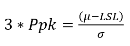
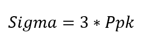
For convenience, let’s assume the equation below:
If we multiply both sides by 3, the equation becomes:
The value on the right side can be expressed as – how many standard deviations are contained in the split process window? This is also the Sigma value or the z-score.
For example, if the Ppk is 1.00, then the z-score is 3.00. This means that the process window and the specification window overlap exactly. This corresponds to 99.73% of the curve. Please note that, I am assuming that the process is perfectly centered here. Refer to this post for additional details on calculations for unilateral and bilateral capabilities.
In other words,
This relationship allows us to estimate the %-conforming (% under the curve) by just knowing the process capability index value. A keen reader may also notice the similarity to tolerance interval calculations. If we go back to the idea that sigma is the number of standard deviations that the split process window can accommodate, then we can replace Sigma with k1 and k2 factors used for the tolerance interval calculations for unilateral and bilateral interval calculations.
A word of caution here is about the switcheroo that happened. The calculations we are doing are based on the normal probability distribution curve, and not the actual process probability distribution curve. The accuracy of our inferences will depend on how close the actual process probability distribution curve matches the beautiful symmetric normal curve.
In today’s post, I am looking at the relationship between capability index (Cpk or Ppk) and Tolerance Intervals. The capability index is tied to the specification limits, and tying this to the tolerance interval allows us to utilize the confidence/reliability statement allowed by the tolerance interval calculation.
Consider the scenario below:
A quality engineer is tasked with assessing the capability of a sealing process. The requirement the engineer is used to is that the process capability index, Ppk, must be greater than or equal to 1.33. The engineer is used to using 30 as the sample size.
But what does this really tell us about the process? Is 1.33 expected to be the population parameter? If so, does testing 30 samples provide us with this information? The capability index calculated from 30 samples is only the statistic and not the parameter.
We can utilize the tolerance interval calculation approach here and calculate the one-sided k-factor for a sample size of 30. Let us assume that we want to find the tolerance interval that will cover 99.9% of the population with 95% confidence. NIST provides us a handy reference to calculate this and we can utilize an Excel spreadsheet to do this for us. We see that the one-sided k-factor calculated is 4.006.
The relationship between the required Ppk and the one-sided k-factor is as follows:
Ppkrequired = k1/3
Similarly for a bilateral specification, the relationship between the required Ppk and the two-sided k-factor is:
Ppkrequired = k2/3
In our example, the required Ppk is 1.34. In other words, if we utilize a sample size of 30 and show that the calculated Ppk is 1.34 or above, we can make the following statement:
With 95% confidence, at least 99.9% of the population is conforming to the specifications. In other words, with 95% confidence, we can claim at least 99.9% reliability.
This approach is also utilized for variable sampling plans. However, please do note that the bilateral specification also requires an additional condition to be met for variable sample plans.
I have attached a spreadsheet that allows the reader to perform these calculations easily. I welcome your thoughts. Please note that the spreadsheet is provided as-is with no guarantees.
Final words:
I will finish with the history of the process capability indices from a great article by Roope M. Turunen and Gregory H. Watson. [1]
The concept of process capability originated in the same Bell Labs group where Walter A. Shewhart developed SPC. Bonnie B. Small led the editing team for the Western Electric Statistical Quality Control Handbook, but the contributor of the process capability concept is not identified. The handbook proposes two methods by which to calculate process capability: first, “as a distribution having a certain center, shape and spread,” and second, “as a percentage outside some specified limit.” These methods were combined to create a ratio of observed variation relative to standard deviation, which is expressed as a percentage. The handbook does not call the ratio an index; this terminology was introduced by two Japanese quality specialists in their 1956 conference paper delivered to the Japanese Society for Quality Control (JSQC). M. Kato and T. Otsu modified Bell Labs’ use of percentage and converted it to an index, and proposed using that as a Cp index to measure machine process capability. Subsequently, in a 1967 JSQC conference paper, T. Ishiyama proposed Cpb as a measurement index of bias in nonsymmetric distributions. This later was changed to Cpk, where “k” refers to the Japanese term katayori, which means “offset” or “bias.”
The title of this post is a nod to the French psychoanalyst, Jacques Lacan[1]. In today’s post, I am looking at the idea of communication. The etymology of “communication” goes back to the Latin words, com and munus. The basic meaning of communication is to make something common. “Com” means “together” while “munus” means “service”, “gift” etc. A closely related word to “communication” is “information”. Similar to “communication”, the etymology of “information” also goes back to its Latin roots. The two Latin words are “in” and “formare”. Taken together, the meaning of “information” is something like – to give shape or form to something. In the context of “information”, this would be – to give shape or form to knowledge or a set of ideas.
In Cybernetics, a core concept is the idea of informational closure. This means that a system such as each one of us is informally closed. Information does not enter into the system. Instead, the system is perturbed by the external world, and based on its interpretative framework, the system finds the perturbation informative.
Informationally closed means that all we have access to is our internal states. For example, when we see a flower, the light hitting the retina of our eyes does not bring in the information that what we are seeing is a flower. Instead, our retinal cells undergo a change of state from the light hitting them. There is nothing qualitative about this interaction. Based on our past interactions and the stability of our experiential knowledge we see the perturbation as informative, and we represent that as “flower”. The word is used to describe a sliver of our experiential reality.
Now this presents a fascinating idea – if we are informationally closed how does communication take place? There can be no direct transfer of information happening between two interacting agents. All that is happening is a relay of perturbations mainly. In order to posit the possibility of communication, the interacting agents should have access to a common set of meanings. When a message is transmitted, both the transmitter and the receiver should be working with a set of possible messages that are contextual. This allows the receiver to choose the most meaningful messages from the set of possible messages. For example, if my friend says that he has a chocolate lab, and I take it to mean that he has a lab where he crafts delectable chocolate creations, then from my friend’s standpoint a miscommunication has occurred. A person more familiar with dogs would have immediately started talking about dogs.
Communication takes place in the form of verbal and nonverbal communication. This adds to the complexity of communication. All communication takes place in a social realm in the background of history of past interactions, cultural norms, language norms, inside jokes etc. Language, as Wittgenstein would say, lies in the public realm. In other words, our private experiences can only be described in terms of public language. Being informationally closed means that we have to indeed work hard at getting good at this communication business. Language is dynamic and ever evolving, and this makes communication even more challenging. Our communication will always be lacking.
I will finish with the wise words of William H. Whyte:
The great enemy of communication, we find, is the illusion of it… we have failed to concede the immense complexity of our society–and thus the great gaps between ourselves and those with whom we seek understanding.
In today’s post, I am looking at absurdity in Systems Thinking. Absurdity is an official term used in the school of philosophy called existentialism. An existentialist believes that existence precedes essence. This means that our essence is not pregiven. Our meaning and purpose are that which we create. In existentialism, the notion of absurdity comes from the predicament that we are by nature meaning makers, and we are thrown into a world devoid of meaning. We do not have direct access to the external world; therefore, our cognitive framework has been tweaked by evolution to seek meaning in all perturbations we encounter. We are forever trying to make sense of a world devoid of any sense or meaning.
We like to imagine that there is greater meaning to this all and that there is a “system” of objective truths in this world. In this framework, we all have access to an objective reality where we can use 2 x 2 matrices to solve complex problems. In the existentialist framework, we see that instead of a “system” of objective truths, we have multiplicity of subjective truths. Soren Kierkegaard, one of the pioneers of existentialism, viewed subjective truth as the highest truth attainable.
When we talk about a “system” we are generally talking about a collection of interrelated phenomena that serves a purpose. From the existentialism standpoint, every “system” is a construction by someone to make sense of something. For example, when I talk about the healthcare system, I have a specific purpose in mind – one that I constructed. The parts of this system serve the purpose of working together for a goal. However, this is my version and my construction. I cannot act as if everyone has the same perspective as me. I could be viewing this as a patient, while someone else, say a doctor, could see an entirely different “system” from their viewpoint. Systems have meaning only from the perspective of a participant or an observer. We are talking about systems as if they have an inherent meaning that is grasped by all. When we talk about fixing “systems”, we again treat a conceptual framework as if they are real things in the world like a machine. The notion of absurdity makes sense here. The first framework is like what Maurice Merleau-Ponty, another existential philosopher, called “high-altitude thinking”. Existentialism rejects this framework. In existentialism, we see that all “systems” are human systems – conceptual frameworks unique to everyone who constructed them based on their worldviews and living experiences. Each “system” is thus highly rich from all aspects of the human condition.
Kevin Aho wrote about this beautifully in the essay, “Existentialism”:
By practicing what Merleau-Ponty disparagingly calls, “high-altitude thinking”, the philosopher adopts a perspective that is detached and impersonal, a “God’s eye view” or “view from nowhere” uncorrupted by the contingencies of our emotions, our embodiment, or the prejudices of our time and place. In this way the philosopher can grasp the “reality” behind the flux of “appearances,” the essential and timeless nature of things “under the perspective of eternity” (sub specie aeternitatis). Existentialism offers a thoroughgoing rejection of this view, arguing that we cannot look down on the human condition from a detached, third-person perspective because we are already thrown into the self-interpreting event or activity of existing, an activity that is always embodied, felt, and historically situated.
We are each thrown here into the world devoid of any meaning, and we try to make meaning. In the act of making sense and meaning, we tend to believe that our version of world and systems are real. We often forget to see the world from others’ viewpoints.
Every post about Systems Thinking must contain the wonderful quote from West Churchman – the systems approach begins when first you see the world through the eyes of another. This beautifully captures the essence of Systems Thinking. Existentialism teaches us to realize the absurdity of seeking meaning in a world devoid of any meaning, while at the same time realizing that the act of seeking meaning itself is meaningful for us.
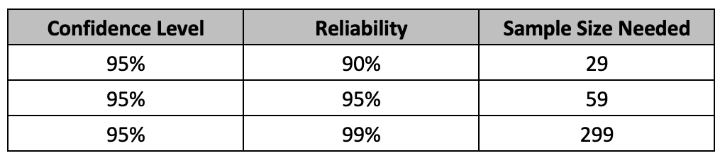
In today’s post, I am looking at some practical suggestions for reducing sample sizes for attribute testing. A sample is chosen to represent a population. The sample size should be sufficient enough to represent the population parameters such as mean, standard deviation etc. Here, we are looking at attribute testing, where a test results in either a pass or a fail. The common way to select an appropriate sample size using reliability and confidence level is based on success run theorem. The often-used sample sizes are shown below. The assumptions for using binomial distribution holds true here.
The formula for the Success Run Theorem is given as:
n = ln(1 – C)/ ln(R), where n is the sample size, ln is the natural logarithm, C is the confidence level and R is reliability.
Selecting a sample size must be based on risk involved. The specific combinations of reliability and confidence level should be tied to the risk involved. Testing for higher risk profile attributes require higher sample sizes. For example, for a high-risk attribute, one can test 299 samples and if there were no rejects found, then claim that at 95% confidence, the product lot is at least 99% conforming or that the process that produced the product is at least 99% reliable.
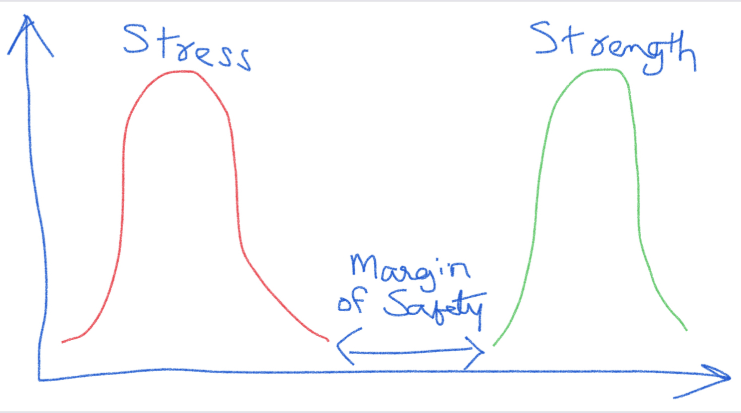
Often time, due to several constraints such as material availability, resource constraints, unforeseen circumstances etc., one may not be able to utilize required sample sizes needed. I am proposing here that we can utilize the stress/strength relationship to appropriately justify the use of a smaller sample size while at the same time not compromise on the desired reliability/confidence level combination.
A common depiction of a stress/strength relationship is shown below for a product. We can see that as long as the stress distribution does not overlap with the strength distribution, the product should function with no issues. The space between the two distributions is referred to as the margin of safety. Often, the product manufacturer defines the normal operating parameters based on this. The specifications for the product are also based on this and some value of margin of safety is incorporated in the specifications.
For example, let’s say that the maximum force that the glue joint of a medical device would see during normal use is 0.50 pound-force, and the specification is set as 1.5 pound-force to account for a margin of safety. It is estimated that a maximum of 1% can likely fail at 1.5 pound-force. This refers to 99% reliability. As part of design verification, we could test 299 samples at 1.5 pound-force and if we do not have any failures, claim that the process is at least 99% reliable at 95% confidence level. If the glue joint is tested at 0.50 pound-force, we should be expecting no product to fail. This is after all, the reason to include the margin of safety.
Following this logic, if we increase the testing stress, we will also increase the likelihood for failures. For example, by increasing the stress five-fold (7.5 pound-force), we are also increasing the likelihood of failure by five-fold (5%) or more. Therefore, if we test 60 parts (one-fifth of 299 from the original study) at 7.5 pound-force and see no failures, this would equate to 99% reliability at 95% confidence at 1.5 pound-force. We can claim at least 99% reliability of performance at 95% confidence level during normal use of product. We were able to reduce the sample size needed to demonstrate the required 99% reliability at 95% confidence level by increasing the stress test condition.
Similarly, if we are to test the glue joint at 3 pound-force (two-fold), we will need 150 samples (half of 299 from the original study) with no failures to claim the same 99% reliability at 95% confidence level during the normal use of product. The rule of thumb is that when aiming for a testing margin of safety of ‘x,’ we can reduce the sample size by a factor of ‘1/x’ while maintaining the same level of reliability and confidence. The exact number can be found by using the success run theorem. In our example, we estimate at least 95% reliability based on the 5% failures while using 5X stress test conditions, when compared to the original 1% failures. Using the equation ln(1-C)/ln(R), where C = 0.95 and R = 0.95, this equates to 59 samples. Similarly for 2X stress conditions, we estimate 2% failures, and here R = 0.98. Using C = 0.95 in the equation, we get the sample size required as 149.
If we had started with a 95% reliability (5% failures utmost) and 95% confidence at the 1X stress conditions, and we go to 2X stress conditions, then we need to calculate the reduced sample size based on 10% failures (2 x 5%). This means that the reliability is estimated to be 90% at 2X stress conditions. Using 0.95 for confidence and 0.90 reliability, this equates to a reduced sample size of 29.
A good resource to follow up on this is Dr. Wayne Taylor’s book, “Statistical Procedures for the Medical Device Industry”. Dr. Taylor notes that:
An attribute stress test results in a pass/fail result. However, the unit is exposed to higher stresses than are typical under normal conditions. As a result, the stress test is expected to produce more failures than will occur under normal conditions. This allows the number of units tested to be reduced. Stress testing requires identifying the appropriate stressor, including time, temperature, force, humidity and voltage. Examples of stress tests include dropping a product from a higher height, exposing a product to more cycles and exposing a product to a wider range of operating conditions.
Many test methods contained in standards are in fact stress tests designed to provide a safety margin. For example, the ASTM packaging standards provide for conditioning units by repeated temperature/humidity cycles and dropping of units from heights that are more extreme and at intervals that are more frequent than most products would typically see during shipping. As a result, it is common practice to test smaller sample sizes. The ASTM packaging conditioning tests are shown… to be five-times stress tests.
It should be apparent that if the product is failing at the elevated stress level, we cannot claim the margin of safety, we were going for. We need to clearly understand how the product will be used in the field and what the normal performance conditions are. We need a good understanding of the safety margins involved. With this approach, if we are able to improve the product design to maximize the safety margins for the specific attributes, we can then utilize a smaller sample size than what is noted in the table above.
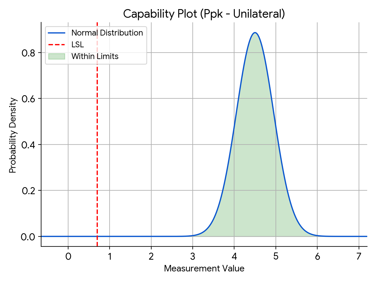
1) It’s commonly used to depict a distribution using +/-3 standard deviations (σ). This is a practical way to visualize a distribution.
2) The most prevalent representation of a distribution often resembles a symmetrical bell curve. However, this is a simplified sketch and not intended to accurately represent the true data distribution, which may exhibit various distribution shapes with varying degrees of fit.
In today’s post, I am explaining how to derive the Success Run Theorem using some basic assumptions. Success Run theorem is one of the most common statistical rational for sample sizes used for attribute data. It goes in the form of:
Having zero failures out of 22 samples, we can be 90% confident that the process is at least 90% reliable (or at least 90% of the population is conforming).
Or
Having zero failures out of 59 samples, we can be 95% confident that the process is at least 95% reliable (or at least of 95% of the population is conforming).
The formula for the Success Run Theorem is given as:
n = ln(1 – C)/ ln(R), where n is the sample size, nl is the natural logarithm, C is the confidence level and R is reliability.
The derivation is fairly straightforward and we can use the multiplication rule of probability to do so. Let’s assume that we have a lot of infinite size and we are testing random samples out of the lot. The infinite size of the lot ensures independence of the samples. If the lot was finite and small then the probability of finding good (conforming) or bad (nonconforming) parts will change from sample to sample, if we are not replacing the tested sample back into the lot.
Let’s assume that q is the conforming rate (probability of finding a good part).
Let us calculate the probability of finding 22 conforming products in a row. In other words, we are testing 22 random samples and we want to find out the probability of finding 22 good parts. This is also the probability of NOT finding any bad product in the 22 random samples. For ease of explanation, let us assume that q = 0.9 or 90%. This rate of conforming product can also be notated as the reliability, R.
Using the multiplication rule of probability:
p(22 conforming products in a row) = 0.9 x 0.9 x 0.9 …… x 0.9 = 0.9 ^22
= 0.10
= 10%
If we find zero rejects in the 22 samples, we are also going to accept the lot. Therefore, this is also the probability of accepting the lot.
The complement of this is the probability of NOT finding 22 conforming products in a row, or the probability of finding at least one nonconforming product in the 22 samples. This is also the probability of rejecting the lot.
p(rejecting the lot) = 1 – p(22 conforming products in a row)
= 1 – 0.10 = 0.90
= 90%
This can be also stated as the CONFIDENCE that if the lot is passing our inspection (if we found zero rejects), then the lot is at least 90% conforming.
In other words, C = 1 – R^n
Or R^n = 1 – C
Taking logarithms of both sides,
n * ln(R) = ln(1 – C)
Or n = ln(1 – C)/ln(R)
Using the example, if we tested 22 samples from a lot, and there were zero rejects then we can with 90% confidence say that the lot is at least 90% conforming. This is also a form of LTPD sampling in Acceptance Sampling. We can get the same results using an OC Curve.
Using a similar approach, we can derive a one-sided nonparametric tolerance interval. If we test 22 samples, then we can say with 90% confidence level that at least 90% of the population is above the smallest value of the samples tested.
Any statistic we calculate should reflect our lack of knowledge of the parameter of the population. The use of confidence/reliability statement is one such way of doing it. I am calling this the epistemic humility dictum:
Any statistical statement we make should reflect our lack of knowledge of the “true” value/nature of the parameter we are interested in.
In my post today, I am looking at the idea of complexity from an existentialist’s viewpoint. An existentialist believes that we, humans, create meanings for ourselves. There is no meaning out there that we do not create. An existentialist would say, from this viewpoint, that complexity is entirely dependent upon an observer, a meaning maker.
We are meaning makers, and we assign meanings to things or situations in terms of possibilities. In other words, the what-is is defined by an observer in terms of what-it-can-be. For example, a door is described by an observer in terms of what it can be used for, in relation to other things in its environment. The door’s meaning is generated in terms of its possibilities. For example, it is something for me to enter or exit a building. The door makes sense to me when it has possibilities in terms of action or relation to other things. This is very similar to the ideas of Gibson, in terms of “affordances”.
In existentialism, there are two concepts that go hand in hand that are relevant here. These are “facticity” and “transcendence”. Facticity refers to the constraints a subject is subjected to. For example, I am a middle-aged male living in the 21st century. I could very well blame my facticity for pretty much any situation in life. Transcendence is realizing that I have freedom to make choices to stand up for myself to transcend my facticity and make meaning of my own existence. We exist in terms of facticity and transcendence. We are thrown into this world and we find ourselves situated amidst the temporal, physical, cultural and social constraints. We could very well say that we have a purpose in this world, one that is prescribed to us as part of facticity or we can refer to ourselves to enable us to transcend our facticity and create our own purposes in the world.
In the context of the post, I am using “facticity” to refer to the constraints and “transcendence” to refer to the possibilities. Going back to complexity and an observer, managing complexity is making sense of “what-is” as the constraints, in terms of “what-it-can-be” as the possibilities. We describe a situation in terms of complexity, when we have to make meaning out of it. We do so to manage the situation – to get something out of it. This is a subject-object relationship in many regards. What the object is, is entirely dependent on what the subject can afford. When one person calls something as complex, they are indicating that the variety of the situation is manifold than what they can absorb. Another subject (observer) can describe the same object as something simple. That subject may choose to focus on only certain attributes of the situation, the attributes that the subject is familiar with. Anything can be called as complex or simple from this regard. As I have noted before, a box of air can be as complex as it can get when one considers the motion of an air particle inside, or as simple as it can get when one considers it as a box of “nothing”. In other words, complexity has no meaning without an observer because the meaning of the situation is introduced by the observer.
A social realm obviously adds more nuance to this simply because there are other meaning-makers involved. Going back to existentialism, we are the subject and at the same time objects for the others in the social realm. Something that has a specific meaning to us can have an entirely different meaning to another person. When we draw a box and call that as a “system”, another person can draw a different box that includes only a portion of my box, and call that as the same “system”. In the social realm, meaning-making should be a social activity as well. It will be a wrong approach to use a prescribed framework to make sense because each of us have different facticities and what possibilities lie within a situation are influenced by these facticities. The essence of these situations cannot be prescribed simply because the essence is brought forth in the social realm by different social beings. A situation is as-is with no complexity inherent to it. It is us who interact with it, and utilize our freedom to assign meaning to it. I will finish off with a great quote from Sartre:
Human reality everywhere encounters resistance and obstacles which it has not created, but these resistances and obstacles have meaning only in and through the free choice which human reality is.