It has been a while since I have posted about Quality Statistics. In today’s post, I will talk about how process capability is connected to percent conforming.
In this post, I will be using Cpk and assuming normality for the sake of simplicity. Please bear in mind that there are multiple ways to calculate process capability, and that not all distributions are normal in nature. The two assumptions help me in explaining this better.
What is Cpk?
The process capability index Cpk is a one shot number that gives you an idea of the capability of the process to center around the nominal specification. It also tells you how much percent conforming product is the process producing. Please note that I am not discussing Cp index in this post.
Cpk is determined as the lower of two values. To simplify, let’s call them Cpklower and Cpkupper.
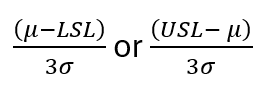
Cpklower = (Process Mean – LSL)/3* s
Cpkupper = (USL – Process Mean)/ 3* s
Where USL is the Upper Specification Limit,
LSL is the Lower Specification Limit, and
s is an estimate of the Population Standard Deviation.
Cpk = minimum (Cpklower, Cpkupper)
The “k” in Cpk stands for “Process Location Ratio” and is dimensionless. It is defined as;
k = abs(Specification Mean – Process Mean)/((USL-LSL)/2)
Where Specification Mean is the nominal specification.
Interestingly when k = 0, Cpk = Cp. This happens when the process is perfectly centered. An additional thing to note is also that Cpk ≈ Ppk when the process is perfectly centered.
You can easily use Ppk in place of Cpk for the above equations. The only difference between Ppk and Cpk is the way we calculate the estimate for the standard deviation.
But What Does Cpk Tell Us?
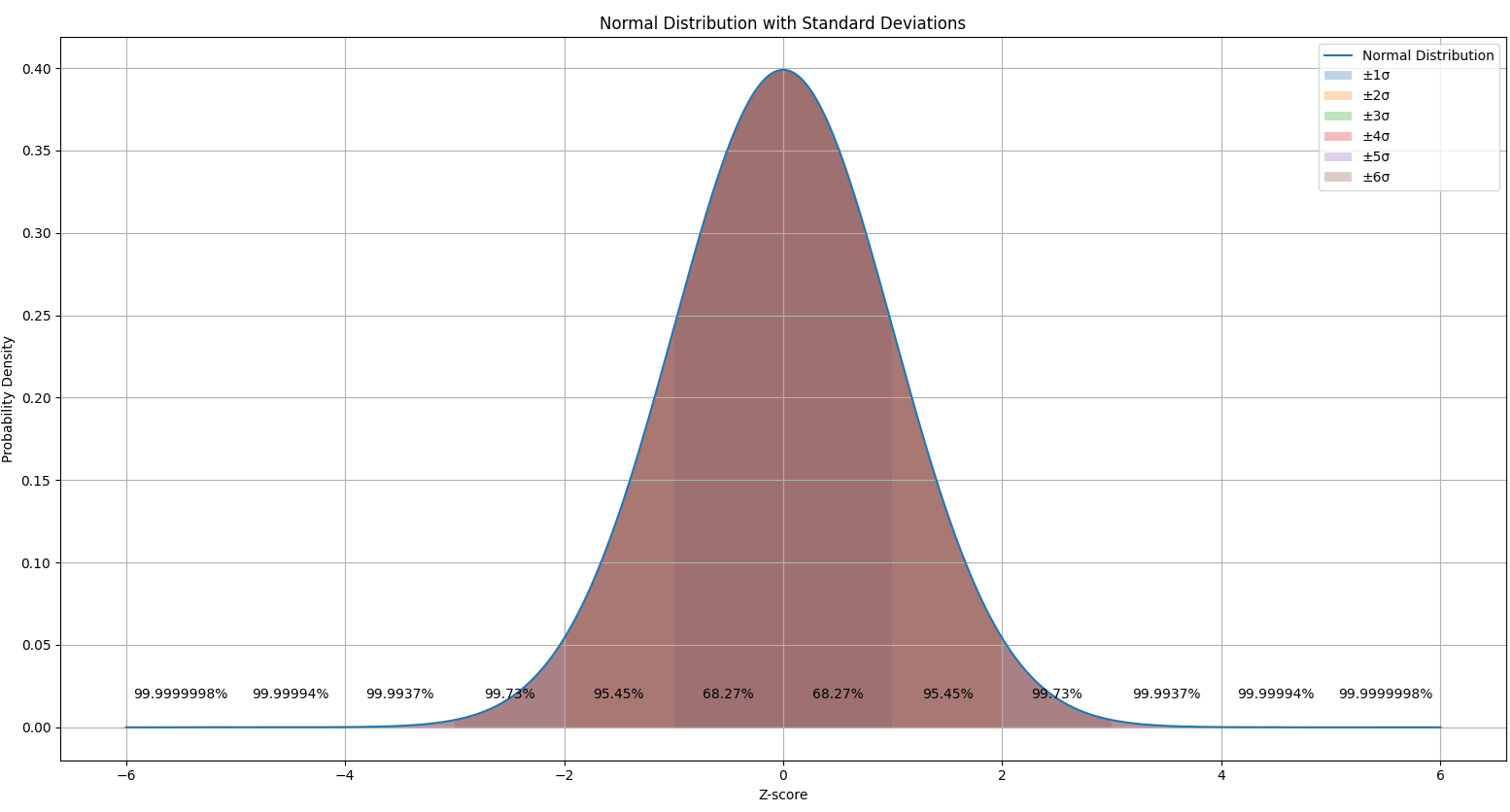
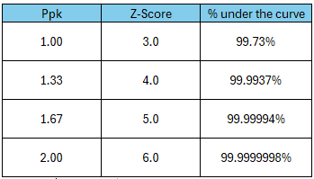
If we can assume normality, we can easily convert the Cpk value to a Z value. This allows one to calculate the percentage falling inside the specification limits using normal distribution tables. We can easily do this in Excel.
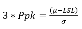
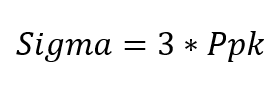
Cpk can be converted to the Z value by simply multiplying it by 3.
Z = 3 * Cpk
In Excel, the Estimated % Non-conforming can be calculated as =NORMSDIST(-Z)
It does get a little tricky, if the process is not centered or if you are looking at a one-sided specification. The table below should come in handy.
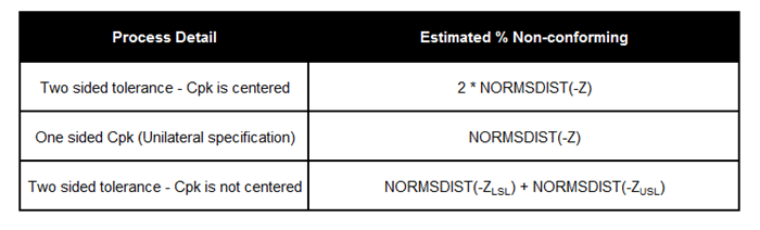
The Estimated % Conforming can be easily calculated as 1 – Estimated % Non-conforming.
The % Conforming is very similar to a tolerance interval calculation. The tolerance interval calculation allows us to make a statement like “we can expect x% of the population to be between two tolerance values at y% confidence level.” However, we cannot make such a statement with just a Cpk calculation. To make such a statement, we will need to calculate the RQL (Rejectable Quality Level) by creating an OC curve. Unfortunately, this is not straightforward, and requires methods like non-central t-distribution. I highly recommend Dr. Taylor’s Distribution Analyzer for this.
What about Confidence Interval?
I am proposing that we can calculate the confidence interval for the Cpk value and thus, for the Estimated % Non-conforming. It is recommended that we use the lower bound confidence interval for this. Before I proceed, I should explain what confidence interval means. It is not technically correct that the population parameter value (e.g. height of kids between ages 10 and 15) is between the two confidence interval bounds. We cannot technically say that at 95% confidence level, the mean height of the population is between X and Y for kids between ages 10 and 15.
Using the mean height as an example, the confidence interval just means that if we keep taking samples from the population, and keep calculating the estimate for mean height, the calculated confidence interval for each of those sample would contain the true mean height, 95% of the time (if we used a 95% confidence level).
We can calculate the lower bound for Cpk at a preferred confidence level, say 95%. We can then convert this to the Z-value and find the estimated % conforming at 95% confidence level. We can then make a statement similar to the tolerance interval.
A Cpk value of 2.00 with a sample size of 12 may not mean much. The calculated Cpk is only an estimate of the true Cpk of the population. Thus like any other parameter (mean, variance etc.), you need a larger sample size to make a better estimate. The use of confidence interval helps us in this regard since it penalizes for lack of sample size.
An Example:
The Quality Engineer at a Medical Device company is performing a capability study on seal strength on pouches. The LSL is 1.1 lbf/in. He used 30 as the sample size, and found that the sample mean was 1.87 lbf/in, and the sample standard deviation was 0.24.
Let’s apply what we have discussed here so far.
LSL = 1.1
Process Mean = 1.87
Process sigma = 0.24
From this we can calculate the Ppk as 1.07. The Quality Engineer calculated Ppk since this was a new process.
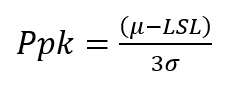
Ppk = (Process Mean – LSL) /3 * Process Sigma
Z = Ppk * 3 = 3.21
Estimated % Non-conforming = NORMSDIST(-Z) = 0.000663675 = 0.07%
Note: Since we are using a unilateral specification, we do not need to double the % non-conforming to capture both sides of the bell curve.
Estimated % Conforming = 1 – Estimated % Non-conforming = 99.93363251%
We can calculate the Ppk lower bound at a 95% confidence level for a sample size = 30. You can use the spreadsheet at the end of this post to do this calculation.
Ppk Lower bound at 95% confidence level = 0.817
Lower bound Z = Ppk_lower_bound x 3 = 2.451
Lower bound (95%) % Non-conforming = NORMSDIST(-Lower_bound_Z) = 0.007122998 = 0.71%
Lower bound (95%) % Conforming = 99.28770023% =99.29%
In effect (all things considered), we can state that with 95% confidence at least 99.29% of the values are in spec. Or we can correctly state that the 95% confidence lower bound for % in spec is 99.29%.
You can download the spreadsheet here. Please note that this post is based on my personal view on the matter. Please use it with caution. I have used normal distribution to calculate the Ppk and the lower bound for Ppk. I welcome your thoughts and comments.
Always keep on learning…
In case you missed it, my last post was Want to Increase Productivity at Your Plant? Read This.