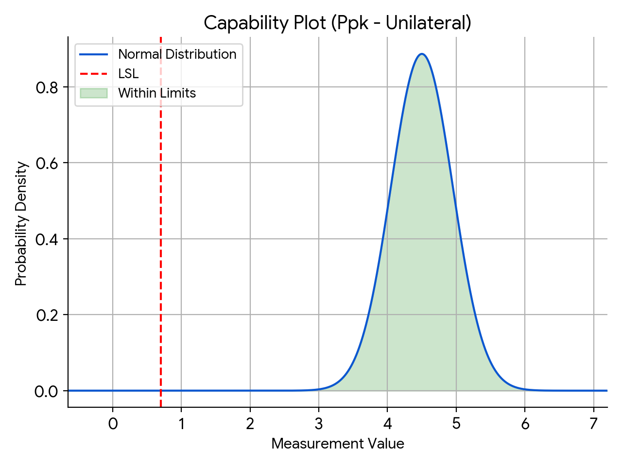
In today’s post, I am looking at the relationship between capability index (Cpk or Ppk) and Tolerance Intervals. The capability index is tied to the specification limits, and tying this to the tolerance interval allows us to utilize the confidence/reliability statement allowed by the tolerance interval calculation.
Consider the scenario below:
A quality engineer is tasked with assessing the capability of a sealing process. The requirement the engineer is used to is that the process capability index, Ppk, must be greater than or equal to 1.33. The engineer is used to using 30 as the sample size.
But what does this really tell us about the process? Is 1.33 expected to be the population parameter? If so, does testing 30 samples provide us with this information? The capability index calculated from 30 samples is only the statistic and not the parameter.
We can utilize the tolerance interval calculation approach here and calculate the one-sided k-factor for a sample size of 30. Let us assume that we want to find the tolerance interval that will cover 99.9% of the population with 95% confidence. NIST provides us a handy reference to calculate this and we can utilize an Excel spreadsheet to do this for us. We see that the one-sided k-factor calculated is 4.006.
The relationship between the required Ppk and the one-sided k-factor is as follows:
Ppkrequired = k1/3
Similarly for a bilateral specification, the relationship between the required Ppk and the two-sided k-factor is:
Ppkrequired = k2/3
In our example, the required Ppk is 1.34. In other words, if we utilize a sample size of 30 and show that the calculated Ppk is 1.34 or above, we can make the following statement:
With 95% confidence, at least 99.9% of the population is conforming to the specifications. In other words, with 95% confidence, we can claim at least 99.9% reliability.
This approach is also utilized for variable sampling plans. However, please do note that the bilateral specification also requires an additional condition to be met for variable sample plans.
I have attached a spreadsheet that allows the reader to perform these calculations easily. I welcome your thoughts. Please note that the spreadsheet is provided as-is with no guarantees.
Final words:
I will finish with the history of the process capability indices from a great article by Roope M. Turunen and Gregory H. Watson. [1]
The concept of process capability originated in the same Bell Labs group where Walter A. Shewhart developed SPC. Bonnie B. Small led the editing team for the Western Electric Statistical Quality Control Handbook, but the contributor of the process capability concept is not identified. The handbook proposes two methods by which to calculate process capability: first, “as a distribution having a certain center, shape and spread,” and second, “as a percentage outside some specified limit.” These methods were combined to create a ratio of observed variation relative to standard deviation, which is expressed as a percentage. The handbook does not call the ratio an index; this terminology was introduced by two Japanese quality specialists in their 1956 conference paper delivered to the Japanese Society for Quality Control (JSQC). M. Kato and T. Otsu modified Bell Labs’ use of percentage and converted it to an index, and proposed using that as a Cp index to measure machine process capability. Subsequently, in a 1967 JSQC conference paper, T. Ishiyama proposed Cpb as a measurement index of bias in nonsymmetric distributions. This later was changed to Cpk, where “k” refers to the Japanese term katayori, which means “offset” or “bias.”
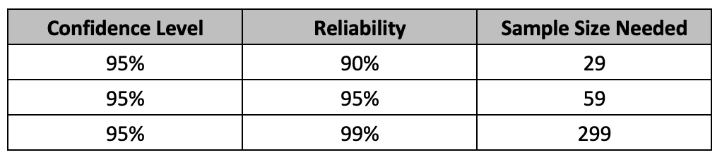
In today’s post, I am looking at some practical suggestions for reducing sample sizes for attribute testing. A sample is chosen to represent a population. The sample size should be sufficient enough to represent the population parameters such as mean, standard deviation etc. Here, we are looking at attribute testing, where a test results in either a pass or a fail. The common way to select an appropriate sample size using reliability and confidence level is based on success run theorem. The often-used sample sizes are shown below. The assumptions for using binomial distribution holds true here.
The formula for the Success Run Theorem is given as:
n = ln(1 – C)/ ln(R), where n is the sample size, ln is the natural logarithm, C is the confidence level and R is reliability.
Selecting a sample size must be based on risk involved. The specific combinations of reliability and confidence level should be tied to the risk involved. Testing for higher risk profile attributes require higher sample sizes. For example, for a high-risk attribute, one can test 299 samples and if there were no rejects found, then claim that at 95% confidence, the product lot is at least 99% conforming or that the process that produced the product is at least 99% reliable.
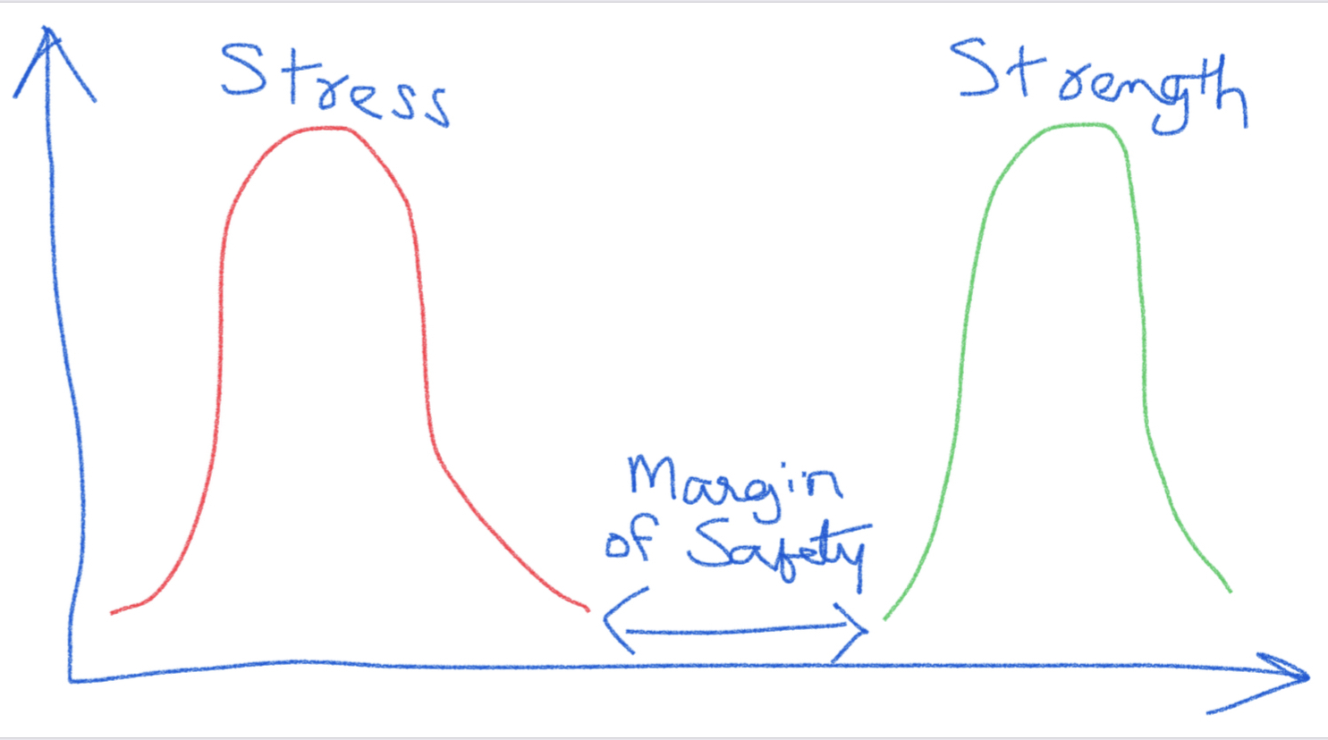
Often time, due to several constraints such as material availability, resource constraints, unforeseen circumstances etc., one may not be able to utilize required sample sizes needed. I am proposing here that we can utilize the stress/strength relationship to appropriately justify the use of a smaller sample size while at the same time not compromise on the desired reliability/confidence level combination.
A common depiction of a stress/strength relationship is shown below for a product. We can see that as long as the stress distribution does not overlap with the strength distribution, the product should function with no issues. The space between the two distributions is referred to as the margin of safety. Often, the product manufacturer defines the normal operating parameters based on this. The specifications for the product are also based on this and some value of margin of safety is incorporated in the specifications.
For example, let’s say that the maximum force that the glue joint of a medical device would see during normal use is 0.50 pound-force, and the specification is set as 1.5 pound-force to account for a margin of safety. It is estimated that a maximum of 1% can likely fail at 1.5 pound-force. This refers to 99% reliability. As part of design verification, we could test 299 samples at 1.5 pound-force and if we do not have any failures, claim that the process is at least 99% reliable at 95% confidence level. If the glue joint is tested at 0.50 pound-force, we should be expecting no product to fail. This is after all, the reason to include the margin of safety.
Following this logic, if we increase the testing stress, we will also increase the likelihood for failures. For example, by increasing the stress five-fold (7.5 pound-force), we are also increasing the likelihood of failure by five-fold (5%) or more. Therefore, if we test 60 parts (one-fifth of 299 from the original study) at 7.5 pound-force and see no failures, this would equate to 99% reliability at 95% confidence at 1.5 pound-force. We can claim at least 99% reliability of performance at 95% confidence level during normal use of product. We were able to reduce the sample size needed to demonstrate the required 99% reliability at 95% confidence level by increasing the stress test condition.
Similarly, if we are to test the glue joint at 3 pound-force (two-fold), we will need 150 samples (half of 299 from the original study) with no failures to claim the same 99% reliability at 95% confidence level during the normal use of product. The rule of thumb is that when aiming for a testing margin of safety of ‘x,’ we can reduce the sample size by a factor of ‘1/x’ while maintaining the same level of reliability and confidence. The exact number can be found by using the success run theorem. In our example, we estimate at least 95% reliability based on the 5% failures while using 5X stress test conditions, when compared to the original 1% failures. Using the equation ln(1-C)/ln(R), where C = 0.95 and R = 0.95, this equates to 59 samples. Similarly for 2X stress conditions, we estimate 2% failures, and here R = 0.98. Using C = 0.95 in the equation, we get the sample size required as 149.
If we had started with a 95% reliability (5% failures utmost) and 95% confidence at the 1X stress conditions, and we go to 2X stress conditions, then we need to calculate the reduced sample size based on 10% failures (2 x 5%). This means that the reliability is estimated to be 90% at 2X stress conditions. Using 0.95 for confidence and 0.90 reliability, this equates to a reduced sample size of 29.
A good resource to follow up on this is Dr. Wayne Taylor’s book, “Statistical Procedures for the Medical Device Industry”. Dr. Taylor notes that:
An attribute stress test results in a pass/fail result. However, the unit is exposed to higher stresses than are typical under normal conditions. As a result, the stress test is expected to produce more failures than will occur under normal conditions. This allows the number of units tested to be reduced. Stress testing requires identifying the appropriate stressor, including time, temperature, force, humidity and voltage. Examples of stress tests include dropping a product from a higher height, exposing a product to more cycles and exposing a product to a wider range of operating conditions.
Many test methods contained in standards are in fact stress tests designed to provide a safety margin. For example, the ASTM packaging standards provide for conditioning units by repeated temperature/humidity cycles and dropping of units from heights that are more extreme and at intervals that are more frequent than most products would typically see during shipping. As a result, it is common practice to test smaller sample sizes. The ASTM packaging conditioning tests are shown… to be five-times stress tests.
It should be apparent that if the product is failing at the elevated stress level, we cannot claim the margin of safety, we were going for. We need to clearly understand how the product will be used in the field and what the normal performance conditions are. We need a good understanding of the safety margins involved. With this approach, if we are able to improve the product design to maximize the safety margins for the specific attributes, we can then utilize a smaller sample size than what is noted in the table above.
1) It’s commonly used to depict a distribution using +/-3 standard deviations (σ). This is a practical way to visualize a distribution.
2) The most prevalent representation of a distribution often resembles a symmetrical bell curve. However, this is a simplified sketch and not intended to accurately represent the true data distribution, which may exhibit various distribution shapes with varying degrees of fit.
In today’s post, I am looking at a topic in Statistics. I have had a lot of feedback on one of my earlier posts on OC curves and how one can use it to generate a reliability/confidence statement based on sample size, n and rejects, c. I provided an Excel spreadsheet that calculates the reliability/confidence based on sample size and rejects. I have been asked how we can utilize Minitab to generate the same results. So, this post is mostly geared towards giving an overview of using OC curves to generate reliability/confidence values and using Minitab to do the same.
The basic premise is that a Type B OC curve can be drawn for samples tested, n and rejects found, c. On the OC curve, the line represents various combinations of reliability and confidence. The OC curve is a plot between percent nonconforming, and probability of acceptance. The lower the percent nonconforming, the higher the probability of acceptance. The probability can be calculated using binomial, hypergeometric or Poisson distributions. The binomial OC curves are called as “Type B” OC curve and do not utilize lot sizes, generally represented as N. The hypergeometric OC curves utilizes lot sizes and are called as “Type A” OC curve. When the ratio n/N is small and n >= 15, the binomial distribution closely matches the hypergeometric distribution. Therefore, the Type B OC curve is used quite often.
The most commonly used standard for attribute sample plans is MIL 105E. The sample plans in MIL 105E are identical to the Z1.4 standard plans. The sampling plans provided as part of the tables do utilize lot sizes. These sampling plans were “tweaked” to include lot sizes because there was a push for including economic considerations of accepting a large lot that may contain rejects. The sample sizes for larger lots were made larger due to this. The OC curves shown in the standards however are Type B OC curves that do not use lot sizes. Hypergeometric distribution considers the fact that there is no replacement for the samples tested. Each test sample removed will impact the subsequent testing since the number of samples is now less. However, as noted above, when the ratio n/N is small, the issue of not replacing samples is not a concern. For the binomial distribution, lot size is not considered since the samples are assumed to be taken from lots of infinite lot size.
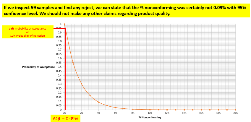
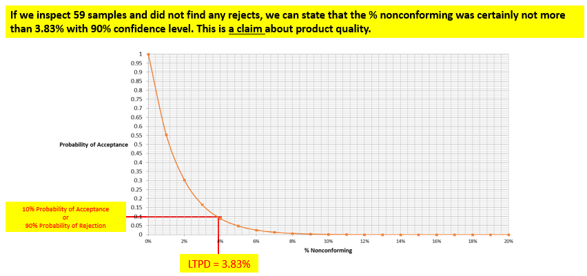
With this background, let’s look at a Type B OC curve. The OC Curve is a plot between % Nonconforming, and Probability of Acceptance. Lower the % Nonconforming, the higher the Probability of Acceptance. The OC Curve shown is for n = 59 with 0 rejects calculated using Binomial Distribution.
The producer’s risk is the risk of good product getting rejected. The acceptance quality limit (AQL) is generally defined as the percent of defectives that the plan will accept 95 percent of the time (i.e., in the long run). Lots that are at or better than the AQL will be accepted 95 percent of the time (in the long run). If the lot fails, we can say with 95-percent confidence that the lot quality level is worse than the AQL. Likewise, we can say that a lot at the AQL that is acceptable has a 5-percent chance of being rejected. In the example, the AQL is 0.09 percent.
The consumer’s risk, on the other hand, is the risk of accepting bad product. The lot tolerance percent defective (LTPD) is generally defined as percent of defective product that the plan will reject 90 percent of the time (in the long run). We can say that a lot at or worse than the LTPD will be rejected 90 percent of the time (in the long run). If the lot passes, we can say with 90-percent confidence that the lot quality is better than the LTPD (i.e., the percent nonconforming is less than the LTPD value). We could also say that a lot at the LTPD that is defective has a 10-percent chance of being accepted.
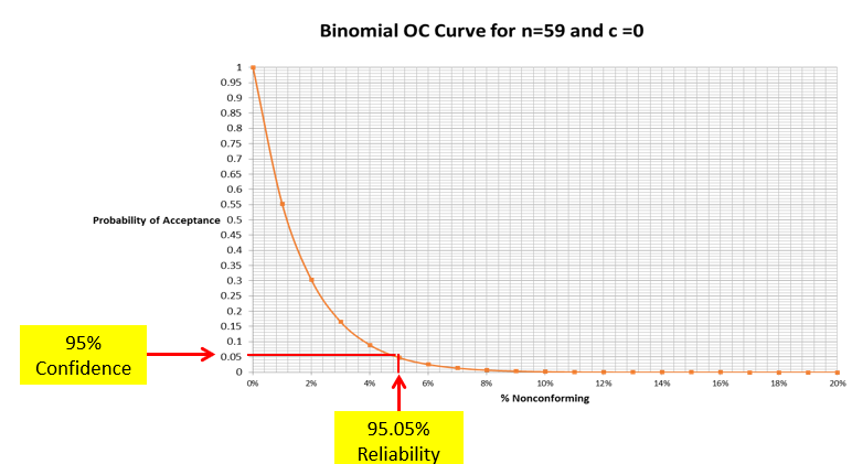
The vertical axis (y axis) of the OC curve goes from 0 percent to 100 percent probability of acceptance. Alternatively, we can say that the y axis corresponds to 100 percent to 0 percent probability of rejection. Let’s call this confidence. This is also the probability of rejecting the lot. The horizontal axis (x axis) of the OC curve goes from 0 percent to 100 percent for percent nonconforming. Alternatively, we can say that the x axis corresponds to 100 percent to 0 percent for percent conforming. Let’s call this reliability.
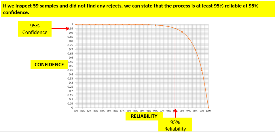
We can easily invert the y axis so that it aligns with a 0 to 100-percent confidence level. In addition, we can also invert the x axis so that it aligns with a 0 to 100-percent reliability level. This is shown below.
The OC Curve line is a combination of reliability and confidence values. Therefore, for any sample size and rejects combination, we can find the required combination of reliability and confidence values. If we know the sample size and rejects, then we can find the confidence value for any reliability value or vice-versa. Let us look at a problem to detail this further:
In the wonderful book Acceptance Sampling in Quality Control by Edward Schilling and Dean Neubauer, the authors discuss a problem that would be of interest here. They posed:
consider an example given by Mann et al. rephrased as follows: Suppose that n = 20 and the observed number of failures is x = 1. What is the reliability π of the units sampled with 90% confidence? Here π is unknown and γ is to be .90.
One of the solutions given was to find the reliability or the confidence desired directly from the OC curve.
They gave the following relation:
π = 1 – p, where π is the reliability and p is the nonconforming rate.
γ = 1 – Pa, where γ is the confidence and Pa is the probability of acceptance.
This is the same relation that was explained above.
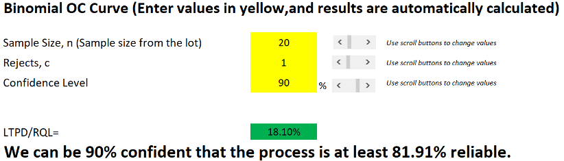
In my spreadsheet, when we enter the values as shown below, we see that the reliability value is 81.91% based on LTPD value of 18.10%. This is the same result documented in the book.
We can use Minitab to get the same result. However, it will be slightly backwards. As I noted above, drawing the OC curve requires only two inputs – the sample size and the number of rejects allowed or acceptance number. Once the OC curve is drawn, we can then look at the different reliability and confidence combinations. We can also calculate the confidence, if we provide the reliability. The reliability is also 1 – p. In Minitab, we can input the sample size, number of rejects and p, and the software will provide us the Pa. For the purpose of reliability and confidence, the p value will be the LTPD value and the confidence value will be 1 – Pa.
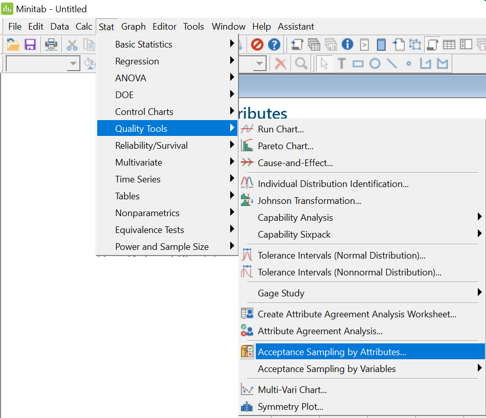
I am using Minitab 18 here. Go to Acceptance Sampling by Attributes as shown below:
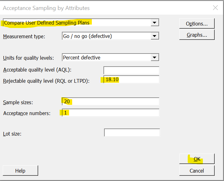
Choose “Compare User Defined Sampling Plans” from the dropdown and enter the different values as shown. Please note that the acceptance number is the maximum number of rejects allowed. Here we are entering the LTPD value because we know the value to be 18.10. In the spreadsheet, we have to enter the confidence level we want to calculate the reliability, while in Minitab we have to enter the LTPD value (1 – reliability) to calculate the confidence. In the example below, we are going to show that entering the LTPD as 18.10 will yield the Pa as 0.10 and thus the confidence as 0.90 or 90%.
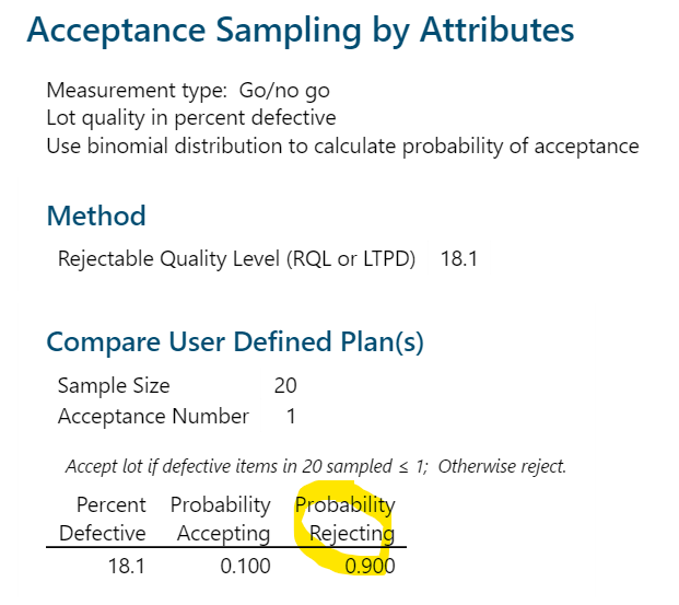
Minitab yields the following result:
One can use the combination of sample size, acceptance number and required LTPD value to calculate the confidence value. The spreadsheet is available here. I will finish with one of the oldest statistical quotes attributed to the famous sixteenth century Spanish writer, Miguel de Cervantes Saavedra that is apt here:
“The proof of the pudding is in the eating. By a small sample we may judge of the whole piece.”
Homer:Every time I have beer on my breath, you assume I’ve been drinking.[1]
In today’s post, I will be looking at process validation and the problem of induction. I have looked at process validation through another philosophical angle by using the lesson of the Ship of Theseus[4] in an earlier post.
US FDA defines process validation [2] as;
“The collection and evaluation of data, from the process design stage through commercial production, which establishes scientific evidence that a process is capable of consistently delivering quality product.”
My emphases on FDA’s definition are the two words – “capability” and “consistency”. One of the misconceptions about process validation is that once the process is validated, then it achieves almost an immaculate status. One of the horror stories I have heard from my friends in the Medical Devices field is that the manufacturer stopped inspecting the product since the process was validated. The problem with validation is the problem of induction. Induction is a process in philosophy – a means to obtain knowledge by looking for patterns from observations and coming to a conclusion. For example, the swans that I have seen so far are white, thus I conclude that ALL swans are white. This is a famous example to show the problem of induction because black swans do exist. However, the data I collected showed that all of the swans in my sample were white. My process of collection and evaluation of the data appears capable and the output consistent.
The misconception that the manufacturer had in the example above was the assumption that the process is going to remain the same and thus the output also will remain the same. This is the assumption that the future and present are going to resemble the past. This type of thinking is termed the assumption of “uniformity of nature” in philosophy. This problem of induction was first thoroughly questioned and looked at by the great Scottish philosopher David Hume (1711-1776). He was an empiricist who believed that knowledge should be based on one’s sense based experience.
One way of looking at process validation is to view the validation as a means to develop a process where it is optimized such that it can withstand the variations of the inputs. Validation is strictly based on the inputs at the time of validation. The 6 inputs – man, machine, method, materials, inspection process and the environment, all can suffer variation as time goes on. These variations reveal the problem of induction – the results are not going to stay the same. There is no uniformity of nature. The uniformities observed in the past are not going to hold for the present and future as well.
In general, when we are doing induction, we should try to meet five conditions;
Use a large sample size that is statistically valid
Make observations under different and extreme circumstances
Ensure that none of the observations/data points contradict
Try to make predictions based on your model
Look for ways and test your model to fail
The use of statistics is considered as a must for process validation. The use of a statistically valid sample size ensures that we make meaningful inferences from the data. The use of different and extreme circumstances is the gist of operational qualification or OQ. OQ is the second qualification phase of process validation. Above all, we should understand how the model works. This helps us to predict how the process works and thus any contradicting data point must be evaluated. This helps us to listen to the process when it is talking. We should keep looking for ways to see where it fails in order to understand the boundary conditions. Ultimately, the more you try to make your model to fail, the better and more refined it becomes.
The FDA’s guidance on process validation [2] and the GHTF (Global Harmonized Task Force) [3] guidance on process validation both try to address the problem of induction through “Continued Process Verification” and “Maintaining a State of Validation”. We should continue monitoring the process to ensure that it remains in a state of validation. Anytime any of the inputs are changed, or if the outputs show a trend of decline, we should evaluate the possibility of revalidation as a remedy for the problem of induction. This brings into mind the quote “Trust but verify”. It is said that Ronald Reagan got this quote from Suzanne Massie, a Russian writer. The original quote is “Doveryai, no proveryai”.
I will finish off with a story from the great Indian epic Mahabharata, which points to the lack of uniformity in nature.
Once a beggar asked for some help from Yudhishthir, the eldest of the Pandavas. Yudhishthir told him to come on the next day. The beggar went away. At the time of this conversation, Yudhishthir’s younger brother Bhima was present. He took one big drum and started walking towards the city, beating the drum furiously. Yudhishthir was surprised.
He asked the reason for this. Bhima told him:
“I want to declare that our revered Yudhishthir has won the battle against time (Kaala). You told that beggar to come the next day. How do you know that you will be there tomorrow? How do you know that beggar would still be alive tomorrow? Even if you both are alive, you might not be in a position to give anything. Or, the beggar might not even need anything tomorrow. How did you know that you both can even meet tomorrow? You are the first person in this world who has won the time. I want to tell the people of Indraprastha about this.”
Yudhishthir got the message behind this talk and called that beggar right away to give the necessary help.