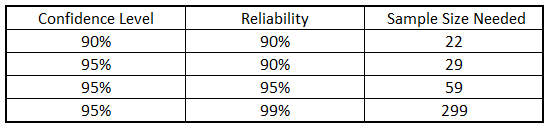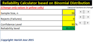
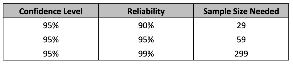
Utilizing Stress/Strength Analysis to Reduce Sample Size:

In today’s post, I am looking at some practical suggestions for reducing sample sizes for attribute testing. A sample is chosen to represent a population. The sample size should be sufficient enough to represent the population parameters such as mean, standard deviation etc. Here, we are looking at attribute testing, where a test results in either a pass or a fail. The common way to select an appropriate sample size using reliability and confidence level is based on success run theorem. The often-used sample sizes are shown below. The assumptions for using binomial distribution holds true here.

The formula for the Success Run Theorem is given as:

n = ln(1 – C)/ ln(R), where n is the sample size, ln is the natural logarithm, C is the confidence level and R is reliability.

Selecting a sample size must be based on risk involved. The specific combinations of reliability and confidence level should be tied to the risk involved. Testing for higher risk profile attributes require higher sample sizes. For example, for a high-risk attribute, one can test 299 samples and if there were no rejects found, then claim that at 95% confidence, the product lot is at least 99% conforming or that the process that produced the product is at least 99% reliable.

Often time, due to several constraints such as material availability, resource constraints, unforeseen circumstances etc., one may not be able to utilize required sample sizes needed. I am proposing here that we can utilize the stress/strength relationship to appropriately justify the use of a smaller sample size while at the same time not compromise on the desired reliability/confidence level combination.

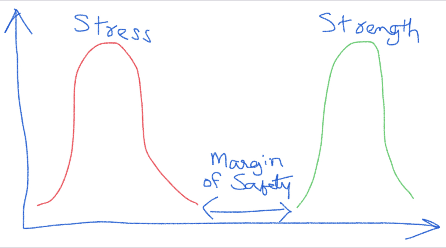
A common depiction of a stress/strength relationship is shown below for a product. We can see that as long as the stress distribution does not overlap with the strength distribution, the product should function with no issues. The space between the two distributions is referred to as the margin of safety. Often, the product manufacturer defines the normal operating parameters based on this. The specifications for the product are also based on this and some value of margin of safety is incorporated in the specifications.

For example, let’s say that the maximum force that the glue joint of a medical device would see during normal use is 0.50 pound-force, and the specification is set as 1.5 pound-force to account for a margin of safety. It is estimated that a maximum of 1% can likely fail at 1.5 pound-force. This refers to 99% reliability. As part of design verification, we could test 299 samples at 1.5 pound-force and if we do not have any failures, claim that the process is at least 99% reliable at 95% confidence level. If the glue joint is tested at 0.50 pound-force, we should be expecting no product to fail. This is after all, the reason to include the margin of safety.

Following this logic, if we increase the testing stress, we will also increase the likelihood for failures. For example, by increasing the stress five-fold (7.5 pound-force), we are also increasing the likelihood of failure by five-fold (5%) or more. Therefore, if we test 60 parts (one-fifth of 299 from the original study) at 7.5 pound-force and see no failures, this would equate to 99% reliability at 95% confidence at 1.5 pound-force. We can claim at least 99% reliability of performance at 95% confidence level during normal use of product. We were able to reduce the sample size needed to demonstrate the required 99% reliability at 95% confidence level by increasing the stress test condition.

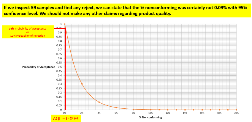
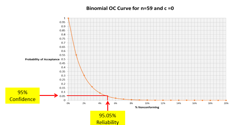
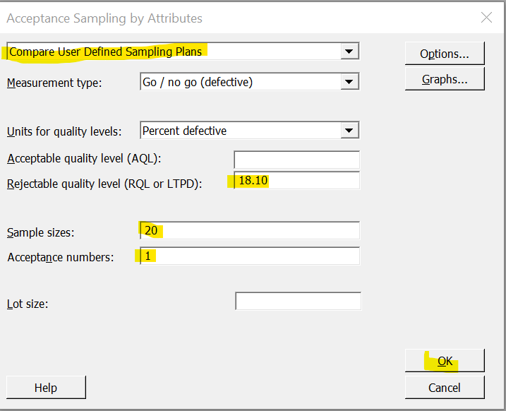
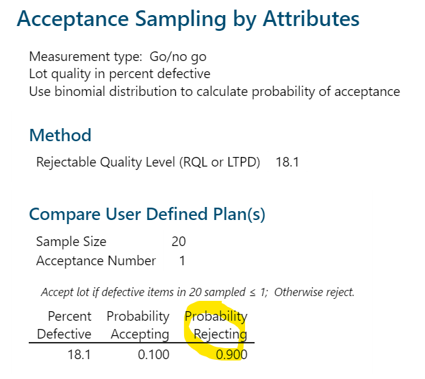
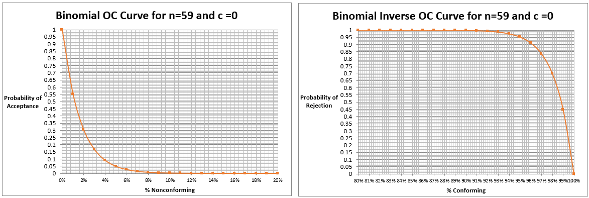
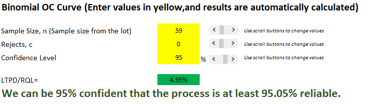
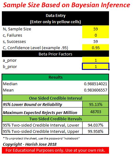
Similarly, if we are to test the glue joint at 3 pound-force (two-fold), we will need 150 samples (half of 299 from the original study) with no failures to claim the same 99% reliability at 95% confidence level during the normal use of product. The rule of thumb is that when aiming for a testing margin of safety of ‘x,’ we can reduce the sample size by a factor of ‘1/x’ while maintaining the same level of reliability and confidence. The exact number can be found by using the success run theorem. In our example, we estimate at least 95% reliability based on the 5% failures while using 5X stress test conditions, when compared to the original 1% failures. Using the equation ln(1-C)/ln(R), where C = 0.95 and R = 0.95, this equates to 59 samples. Similarly for 2X stress conditions, we estimate 2% failures, and here R = 0.98. Using C = 0.95 in the equation, we get the sample size required as 149.

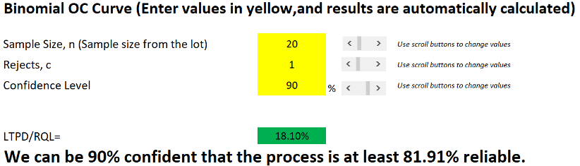
If we had started with a 95% reliability (5% failures utmost) and 95% confidence at the 1X stress conditions, and we go to 2X stress conditions, then we need to calculate the reduced sample size based on 10% failures (2 x 5%). This means that the reliability is estimated to be 90% at 2X stress conditions. Using 0.95 for confidence and 0.90 reliability, this equates to a reduced sample size of 29.

A good resource to follow up on this is Dr. Wayne Taylor’s book, “Statistical Procedures for the Medical Device Industry”. Dr. Taylor notes that:

An attribute stress test results in a pass/fail result. However, the unit is exposed to higher stresses than are typical under normal conditions. As a result, the stress test is expected to produce more failures than will occur under normal conditions. This allows the number of units tested to be reduced. Stress testing requires identifying the appropriate stressor, including time, temperature, force, humidity and voltage. Examples of stress tests include dropping a product from a higher height, exposing a product to more cycles and exposing a product to a wider range of operating conditions.

Many test methods contained in standards are in fact stress tests designed to provide a safety margin. For example, the ASTM packaging standards provide for conditioning units by repeated temperature/humidity cycles and dropping of units from heights that are more extreme and at intervals that are more frequent than most products would typically see during shipping. As a result, it is common practice to test smaller sample sizes. The ASTM packaging conditioning tests are shown… to be five-times stress tests.

It should be apparent that if the product is failing at the elevated stress level, we cannot claim the margin of safety, we were going for. We need to clearly understand how the product will be used in the field and what the normal performance conditions are. We need a good understanding of the safety margins involved. With this approach, if we are able to improve the product design to maximize the safety margins for the specific attributes, we can then utilize a smaller sample size than what is noted in the table above.

Always keep on learning. In case you are interested, my last post was Deriving the Success Run Theorem:

Note:

1) It’s commonly used to depict a distribution using +/-3 standard deviations (σ). This is a practical way to visualize a distribution.

2) The most prevalent representation of a distribution often resembles a symmetrical bell curve. However, this is a simplified sketch and not intended to accurately represent the true data distribution, which may exhibit various distribution shapes with varying degrees of fit.

OC Curve and Reliability/Confidence Sample Sizes:

_{“Reliability” as dreamt by Dream by WOMBO}

In today’s post, I am looking at a topic in Statistics. I have had a lot of feedback on one of my earlier posts on OC curves and how one can use it to generate a reliability/confidence statement based on sample size, n and rejects, c. I provided an Excel spreadsheet that calculates the reliability/confidence based on sample size and rejects. I have been asked how we can utilize Minitab to generate the same results. So, this post is mostly geared towards giving an overview of using OC curves to generate reliability/confidence values and using Minitab to do the same.

The basic premise is that a Type B OC curve can be drawn for samples tested, n and rejects found, c. On the OC curve, the line represents various combinations of reliability and confidence. The OC curve is a plot between percent nonconforming, and probability of acceptance. The lower the percent nonconforming, the higher the probability of acceptance. The probability can be calculated using binomial, hypergeometric or Poisson distributions. The binomial OC curves are called as “Type B” OC curve and do not utilize lot sizes, generally represented as N. The hypergeometric OC curves utilizes lot sizes and are called as “Type A” OC curve. When the ratio n/N is small and n >= 15, the binomial distribution closely matches the hypergeometric distribution. Therefore, the Type B OC curve is used quite often.

The most commonly used standard for attribute sample plans is MIL 105E. The sample plans in MIL 105E are identical to the Z1.4 standard plans. The sampling plans provided as part of the tables do utilize lot sizes. These sampling plans were “tweaked” to include lot sizes because there was a push for including economic considerations of accepting a large lot that may contain rejects. The sample sizes for larger lots were made larger due to this. The OC curves shown in the standards however are Type B OC curves that do not use lot sizes. Hypergeometric distribution considers the fact that there is no replacement for the samples tested. Each test sample removed will impact the subsequent testing since the number of samples is now less. However, as noted above, when the ratio n/N is small, the issue of not replacing samples is not a concern. For the binomial distribution, lot size is not considered since the samples are assumed to be taken from lots of infinite lot size.

With this background, let’s look at a Type B OC curve. The OC Curve is a plot between % Nonconforming, and Probability of Acceptance. Lower the % Nonconforming, the higher the Probability of Acceptance. The OC Curve shown is for n = 59 with 0 rejects calculated using Binomial Distribution.

The producer’s risk is the risk of good product getting rejected. The acceptance quality limit (AQL) is generally defined as the percent of defectives that the plan will accept 95 percent of the time (i.e., in the long run). Lots that are at or better than the AQL will be accepted 95 percent of the time (in the long run). If the lot fails, we can say with 95-percent confidence that the lot quality level is worse than the AQL. Likewise, we can say that a lot at the AQL that is acceptable has a 5-percent chance of being rejected. In the example, the AQL is 0.09 percent.

The consumer’s risk, on the other hand, is the risk of accepting bad product. The lot tolerance percent defective (LTPD) is generally defined as percent of defective product that the plan will reject 90 percent of the time (in the long run). We can say that a lot at or worse than the LTPD will be rejected 90 percent of the time (in the long run). If the lot passes, we can say with 90-percent confidence that the lot quality is better than the LTPD (i.e., the percent nonconforming is less than the LTPD value). We could also say that a lot at the LTPD that is defective has a 10-percent chance of being accepted.

The vertical axis (y axis) of the OC curve goes from 0 percent to 100 percent probability of acceptance. Alternatively, we can say that the y axis corresponds to 100 percent to 0 percent probability of rejection. Let’s call this confidence. This is also the probability of rejecting the lot. The horizontal axis (x axis) of the OC curve goes from 0 percent to 100 percent for percent nonconforming. Alternatively, we can say that the x axis corresponds to 100 percent to 0 percent for percent conforming. Let’s call this reliability.

We can easily invert the y axis so that it aligns with a 0 to 100-percent confidence level. In addition, we can also invert the x axis so that it aligns with a 0 to 100-percent reliability level. This is shown below.

The OC Curve line is a combination of reliability and confidence values. Therefore, for any sample size and rejects combination, we can find the required combination of reliability and confidence values. If we know the sample size and rejects, then we can find the confidence value for any reliability value or vice-versa. Let us look at a problem to detail this further:

In the wonderful book Acceptance Sampling in Quality Control by Edward Schilling and Dean Neubauer, the authors discuss a problem that would be of interest here. They posed:

consider an example given by Mann et al. rephrased as follows: Suppose that n = 20 and the observed number of failures is x = 1. What is the reliability π of the units sampled with 90% confidence? Here π is unknown and γ is to be .90.

One of the solutions given was to find the reliability or the confidence desired directly from the OC curve.

They gave the following relation:

π = 1 – p, where π is the reliability and p is the nonconforming rate.

γ = 1 – P_a, where γ is the confidence and P_ais the probability of acceptance.

This is the same relation that was explained above.

In my spreadsheet, when we enter the values as shown below, we see that the reliability value is 81.91% based on LTPD value of 18.10%. This is the same result documented in the book.

We can use Minitab to get the same result. However, it will be slightly backwards. As I noted above, drawing the OC curve requires only two inputs – the sample size and the number of rejects allowed or acceptance number. Once the OC curve is drawn, we can then look at the different reliability and confidence combinations. We can also calculate the confidence, if we provide the reliability. The reliability is also 1 – p. In Minitab, we can input the sample size, number of rejects and p, and the software will provide us the P_a. For the purpose of reliability and confidence, the p value will be the LTPD value and the confidence value will be 1 – P_a.

I am using Minitab 18 here. Go to Acceptance Sampling by Attributes as shown below:

Choose “Compare User Defined Sampling Plans” from the dropdown and enter the different values as shown. Please note that the acceptance number is the maximum number of rejects allowed. Here we are entering the LTPD value because we know the value to be 18.10. In the spreadsheet, we have to enter the confidence level we want to calculate the reliability, while in Minitab we have to enter the LTPD value (1 – reliability) to calculate the confidence. In the example below, we are going to show that entering the LTPD as 18.10 will yield the P_a as 0.10 and thus the confidence as 0.90 or 90%.

Minitab yields the following result:

One can use the combination of sample size, acceptance number and required LTPD value to calculate the confidence value. The spreadsheet is available here. I will finish with one of the oldest statistical quotes attributed to the famous sixteenth century Spanish writer, Miguel de Cervantes Saavedra that is apt here:

“The proof of the pudding is in the eating. By a small sample we may judge of the whole piece.”

Stay safe and always keep on learning…

In case you missed it, my last post was Second Order Variety:

AQL/RQL/LTPD/OC Curve/Reliability and Confidence:

It has been a while since I have posted about statistics. In today’s post, I am sharing a spreadsheet that generates an OC Curve based on your sample size and the number of rejects. I get asked a lot about a way to calculate sample sizes based on reliability and confidence levels. I have written several posts before. Check this post and this post for additional details.

The spreadsheet is hopefully straightforward to use. The user has to enter data in the required yellow cells.

A good rule of thumb is to use 95% confidence level, which also corresponds to 0.05 alpha. The spreadsheet will plot two curves. One is the standard OC curve, and the other is an inverse OC curve. The inverse OC curve has the probability of rejection on the Y-axis and % Conforming on the X-axis. These corresponds to Confidence level and Reliability respectively.

I will discuss the OC curve and how we can get a statement that corresponds to a Reliability/Confidence level from the OC curve.

The OC Curve is a plot between % Nonconforming, and Probability of Acceptance. Lower the % Nonconforming, the higher the Probability of Acceptance. The probability can be calculated using Binomial, Hypergeometric or Poisson distributions. The OC Curve shown is for n = 59 with 0 rejects calculated using Binomial Distribution.

The Producer’s risk is the risk of good product getting rejected. The Acceptance Quality Limit (AQL) is generally defined as the percent defectives that the plan will accept 95% of the time (in the long run). Lots that are at or better than the AQL will be accepted 95% of the time (in the long run). If the lot fails, we can say with 95% confidence that the lot quality level is worse than the AQL. Likewise, we can say that a lot at the AQL that is acceptable has a 5% chance of being rejected. In the example, the AQL is 0.09%.

The Consumer’s risk, on the other hand, is the risk of accepting bad product. The Lot Tolerance Percent Defective (LTPD) is generally defined as percent defective that the plan will reject 90% of the time (in the long run). We can say that a lot at or worse than the LTPD will be rejected 90% of the time (in the long run). If the lot passes, we can say with 90% confidence that the lot quality is better than the LTPD (% nonconforming is less than the LTPD value). We could also say that a lot at the LTPD that is defective has a 10% chance of being accepted.

The vertical axis (Y-axis) of the OC Curve goes from 0% to 100% Probability of Acceptance. Alternatively, we can say that the Y-axis corresponds to 100% to 0% Probability of Rejection. Let’s call this Confidence.

The horizontal axis (X-axis) of the OC Curve goes from 0% to 100% for % Nonconforming. Alternatively, we can say that the X-axis corresponds to 100% to 0% for % Conforming. Let’s call this Reliability.

We can easily invert the Y-axis so that it aligns with a 0 to 100% confidence level. In addition, we can also invert the X-axis so that it aligns with a 0 to 100% reliability level. This is shown below.

What we can see is that, for a given sample size and defects, the more reliability we try to claim, the less confidence we can assume. For example, in the extreme case, 100% reliability lines up with 0% confidence.

I welcome the reader to play around with the spreadsheet. I am very much interested in your feedback and questions. The spreadsheet is available here.

In case you missed it, my last post was Nature of Order for Conceptual Models:

MTTF Reliability, Cricket and Baseball:

I originally hail from India, which means that I was eating, drinking and sleeping Cricket at least for a good part of my childhood. Growing up, I used to “get sick” and stay home when the one TV channel that we had broadcasted Cricket matches. One thing I never truly understood then was how the batting average was calculated in Cricket. The formula is straightforward:

Batting average = Total Number of Runs Scored/ Total Number of Outs

Here “out” indicates that the batsman had to stop his play because he was unable to keep his wicket. In Baseball terms, this will be similar to a strike out or a catch where the player has to leave the field. The part that I could not understand was when the Cricket batsman did not get out. The runs he scored was added to the numerator but there was no changes made to the denominator. I could not see this as a true indicator of the player’s batting average.

When I started learning about Reliability Engineering, I finally understood why the batting average calculation was bothering me. The way the batting average in Cricket is calculated is very similar to the MTTF (Mean Time To Failure) calculation. MTTF is calculated as follows:

MTTF = Total time on testing/Number of failures

For a simple example, if we were testing 10 motors for 100 hours and three of them failed at 50, 60 and 70 hours respectively, we can calculate MTTF as 293.33 hours. The problem with this is that the data is a right-censored data. This means that we still have samples where the failure has not occurred and we stopped the testing. This is similar to the case where we do not include the number of innings where the batsman did not get out. A key concept to grasp here is that the MTTF or the MTBF (Mean Time Between Failure) metric is not for a single unit. There is more to this than just saying that on average a motor is going to last 293.33 hours.

When we do reliability calculations, we should be aware whether censored data is being used and use appropriate survival analysis to make a “reliability specific statement” – we can expect that 95% of the motor population will survive x hours. Another good approach is to calculate the lower bound confidence intervals based on the MTBF. A good resource is https://www.itl.nist.gov/div898/handbook/apr/section4/apr451.htm.

Ty Cobb. Don Bradman and Sachin Tendulkar:

We can compare the batting averages in Cricket to Baseball. My understanding is that the batting average in Baseball is calculated as follows:

Batting Average = Number of Hits/Number of Bats

Here the hit can be in the form of singles, home runs etc. Apparently, this statistic was initially brought up by an English statistician Henry Chadwick. Chadwick was a keen Cricket fan.

I want to now look at the greats of Baseball and Cricket, and look at a different approach to their batting capabilities. I have chosen Ty Cobb, Don Bradman and Sachin Tendulkar for my analyses. Ty Cobb has the largest Baseball batting average in American Baseball. Don Bradman, an Australian Cricketer often called the best Cricket player ever, has the largest batting average in Test Cricket. Sachin Tendulkar, an Indian Cricketer and one of the best Cricket players of recent times, has the largest number of runs scored in Test Cricket. The batting averages of the three players are shown below:

As we discussed in the last post regarding calculating reliability with Bayesian approach, we can make reliability statements in place of batting averages. Based on 4191 hits in 11420 bats, we could make a statement that – with 95% confidence Ty Cobb is 36% likely to make a hit in the next bat. We can utilize the batting average concept in Baseball to Cricket. In Cricket, hitting fifty runs is a sign of a good batsman. Bradman has hit fifty or more runs on 56 occasions in 80 innings (70%). Similarly Tendulkar has hit fifty or more runs on 125 occasions in 329 innings (38%).

We could state that with 95% confidence, Bradman was 61% likely to score fifty or more runs in the next inning. Similarly, Sachin was 34% likely to score fifty runs or more in the next inning at 95% confidence level.

Final Words:

As we discussed earlier, similar to MTTF, batting average is not a good estimation for a single inning. It is an attempt for a point estimate for reliability but we need additional information regarding this. This should not be looked at it as a single metric in isolation. We cannot expect that Don Bradman would score 99.94 runs per innings. In fact, in the last very match that Bradman played, all he had to do was score 4 single runs to achieve the immaculate batting average of 100. He had been out only 69 times and he just needed four measly runs to complete 7000 runs and even if he got out on that inning, he would have achieved the spectacular batting average of 100. He was one of the best players ever. His highest score was 334. This is called “triple century” in Cricket, and this is a rare achievement. As indicated earlier, he was 61% likely to have scored fifty runs or more in the next inning. In fact, Bradman had scored more than four runs 69 times in 79 innings.

Everyone expected Bradman to cross the 100 mark easily. As fate would have it, Bradman scored zero runs as he was bowled out (the batsman misses and the ball hits the wicket) by the English bowler Eric Hollies, in the second ball he faced. He had hit 635 fours in his career. A four is where the batsman scores four runs by hitting the ball so that it rolls over the boundary of the field. All Bradman needed was one four to achieve the “100”. Bradman proved that to be human is to be fallible. He still remains the best that ever was and his record is far from broken. At this time, the batsman with the second best batting average is 61.87.

Always keep on learning…

In case you missed it, my last post was Reliability/Sample Size Calculation Based on Bayesian Inference:

Reliability/Sample Size Calculation Based on Bayesian Inference:

I have written about sample size calculations many times before. One of the most common questions a statistician is asked is “how many samples do I need – is a sample size of 30 appropriate?” The appropriate answer to such a question is always – “it depends!”

In today’s post, I have attached a spreadsheet that calculates the reliability based on Bayesian Inference. Ideally, one would want to have some confidence that the widgets being produced is x% reliable, or in other words, it is x% probable that the widget would function as intended. There is the ubiquitous 90/90 or 95/95 confidence/reliability sample size table that is used for this purpose.

In Bayesian Inference, we do not assume that the parameter (the value that we are calculating like Reliability) is fixed. In the non-Bayesian (Frequentist) world, the parameter is assumed to be fixed, and we need to take many samples of data to make an inference regarding the parameter. For example, we may flip a coin 100 times and calculate the number of heads to determine the probability of heads with the coin (if we believe it is a loaded coin). In the non-Bayesian world, we may calculate confidence intervals. The confidence interval does not provide a lot of practical value. My favorite explanation for confidence interval is with the analogy of an archer. Let’s say that the archer shot an arrow and it hit the bulls-eye. We can draw a 3” circle around this and call that as our confidence interval based on the first shot. Now let’s assume that the archer shot 99 more arrows and they all missed the bull-eye. For each shot, we drew a 3” circle around the hit resulting in 100 circles. A 95% confidence interval simply means that 95 of the circles drawn contain the first bulls-eye that we drew. In other words, if we repeated the study a lot of times, 95% of the confidence intervals calculated will contain the true parameter that we are after. This would indicate that the one study we did may or may not contain the true parameter. Compared to this, in the Bayesian world, we calculate the credible interval. This practically means that we can be 95% confident that the parameter is inside the 95% credible interval we calculated.

In the Bayesian world, we can have a prior belief and make an inference based on our prior belief. However, if your prior belief is very conservative, the Bayesian inference might make a slightly liberal inference. Similarly, if your prior belief is very liberal, the inference made will be slightly conservative. As the sample size goes up, impact of this prior belief is minimized. A common method in Bayesian inference is to use the uninformed prior. This means that we are assuming equal likelihood for all the events. For a binomial distribution we can use beta distribution to model our prior belief. We will use (1, 1) to assume the uninformed prior. This is shown below:

For example, if we use 59 widgets as our samples and all of them met the inspection criteria, then we can calculate the 95% lower bound credible interval as 95.13%. This is assuming the (1, 1) beta values. Now let’s say that we are very confident of the process because we have historical data. Now we can assume a stronger prior belief with the beta values as (22,1). The new prior plot is shown below:

Based on this, if we had 0 rejects for the 59 samples, then the 95% lower bound credible interval is 96.37%. A slightly higher reliability is estimated based on the strong prior.

We can also calculate a very conservative case of (1, 22) where we assume very low reliability to begin with. This is shown below:

Now when we have 0 rejects with 59 samples, we are pleasantly surprised because we were expecting our reliability to be around 8-10%. The newly calculated 95% lower bound credible interval is 64.9%.

I have created a spreadsheet that you can play around with. Enter the data in the yellow cells. For a stronger prior (liberal), enter a higher a_prior value. Similarly, for a conservative prior, enter a higher b_prior value. If you are unsure, retain the (1, 1) value to have a uniform prior. The spreadsheet also calculates the maximum expected rejects per million value as well.

You can download the spreadsheet here.

I will finish with my favorite confidence interval joke.

“Excuse me, professor. Why do we always calculate 95% confidence interval and not a 94% or 96% interval?”, asked the student.

“Shut up,” explained the professor.

Always keep on learning…

In case you missed it, my last post was Mismatched Complexity and KISS:

Reliability/Confidence Level Calculator (with c = 0, 1….., n)

The reliability/Confidence level sample size calculation is fairly known to Quality Engineers. For example, with 59 samples and 0 rejects, one can be 95% confident that the process is at least 95% reliable or that the process yields at least 95% conforming product.

I have created a spreadsheet “calculator”, that allows the user to enter the sample size, number of rejects and the desired confidence level, and the calculator will provide the reliability result.

It is interesting to note that the reliability/confidence calculation, LTPD calculation and Wilk’s first degree non-parametric one sided tolerance calculation all yield the same results.

I will post another day about LTPD versus AQL.

The spreadsheet is available here Reliability calculator based on Binomial distribution.

I have a new post in this topic. Check out https://harishsnotebook.wordpress.com/2019/10/19/aql-rql-ltpd-oc-curve-reliability-and-confidence/

Keep on learning…

Wilk’s One Sided Tolerance spreadsheet for download

I have created a spreadsheet that allows the user to calculate the number of samples needed for a desired one-sided tolerance interval at a desired confidence level. Additionally, the user can also enter the desired order for the sample size.

For example, if you have 93 samples, you can be 95% confident that 95% of the population are above the 2nd lowest value samples. Alternatively, you can also state that 95% of the population is below the 2nd highest value of the samples.

Here is an example of this in use.

If there is an interest, I can also try creating a two sided tolerance interval spreadsheet as well.

The keen student might notice that the formula is identical to the Bayes Success Run Theorem when the order p =1.

The spreadsheet is available for download here. Wilks one sided

Keep on learning…

Harish's Notebook – My notes… Lean, Cybernetics, Quality & Data Science.

Menu

Tag Archives: Sample Size